Image Measurements and Refinements

Introduction:

The solution for most photogrammetric problems involves some photographic measurements. Sometimes the measurement is just the length of lines between imaged points or by row and column method to define the pixel location, and if the dimension of the pixel is known then this method can b. Converted into a linear coordinate this will create a left handed coordinate system which may cause some calculation problems. but the most common system is the rectangular coordinate, and it used directly in many photogrammetric equations. Image measurement can be done on a positive photo printed in a paper, glass, film or it can be manipulated digitally on a computer. It also can be made on negative photos but it is better to preserve the negative in case more positive may be printed because it may deface the negative. Also sometimes scanned negative into a digital from to prevent any additional cost for making positive images. Some errors occur during the process of image measurement the major source of the errors are:

1. Film distortions due to shrinkage, expansion, and lack of flatness.

2. CCD array distortions due to electrical signal timing issues or lack of flatness of the chip surface.

3. Failure of photo coordinate axes to intersect at the principal point.

4. Failure of principal point to be aligned with centre of CCD array.

5. Lens distortions.

6. Atmospheric refraction distortions.

7. Earth curvature distortion.

Image measurement coordinate system:

The rectangular coordinate system specifies the point location by it is rectangular distance from the axes. X axis is defined arbitrary by a straight line connecting the opposite fiducial points along the flight direction. x axis is positive and parallel with the flight direction. The y axis is 90 degree counterclockwise from the positive x axis. The two axis x , y intersect in a point called the principal point. The principal point is the origin of the rectangular coordinate system which is a right hand coordinate system. The principal point will be near to the true principal point of the image if not -due to the fact that fiducial points are slightly not in the exact opposite direction of each other- it may cause some systematic errors so that some refinement will be applied to make them corresponding with the use of fiducial points as a control points. The next figure shows this system and how a coordinate of points a, b can be defined.

The rectangular coordinate system with the use of simple analytical geometry some calculations are very useful. Such as the imaged distance between point a and b can be calculated from:

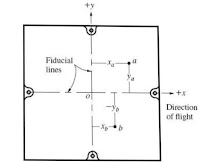
Image measurement instruments:

The instruments used in photogrammetric measurements varies depending on the accuracy needed from simple scales on analogue maps to computers on digital maps:

1. Simple Scales:

There are different types of scales depending on the accuracy demanded for the problem at hand. If a low accuracy is good then a simple engineer’s scales can be used, and there accuracy can be enhanced by using magnifying glasses with right graduation as long as taking care while measuring. Engineering scales are available in both metric and English units. In greater accuracy a device such as the glass scale can be used.

2. Comparator:

Comparator provide the ultimate accuracy in the direct measurement of film  typically 2 or 3 micrometre and they are used to camera calibration and analytical photogrammetry. they are no longer in use and they so called comparator because it compare the photographic position of imaged points in respect to the measurement scales of the devices. There are two basic types of comparators:

1. Monocomparators: they make measurement on one photograph at a time. They no longer manufactured.

2. Stereocomparators: they make measurement by simultaneously viewing an overlap pair of photographs.

The analytical Stereoplotter is commonly used to do the function of both Monocomparators and Stereocomparators.

3. Photogrammetric Scanners:

They are devices that convert the content of photographers from its analogue form to a digital form (an array of pixel that contain a digital number). Once the image is in digital form, the coordinate measurement can either be by a help of human or automate algorithm. Photogrammetric scanners are less manufactured due to the use of digital cameras. Although there are deferent approaches but they all have the same fundamental concept. It is essential that the scanner has a good geometric and radio metric resolution as well as geometric accuracy.

Geometric or spatial resolution is an indication of the pixel size. The small size of a pixel the great details an image can provide. Quality scanners are capable of producing a minimum of 5 to 15 micrometre pixel size. Radiometric resolution is an indication of the number of quantization levels assosiated with a single pixel. Minimum radiometric resolution is 256 levels (8-bit), most scanners are capable of  1024 levels (10-bit).

Refinement of Measured Image Coordinate:

Correction can be applied to eliminate the effect of systematic errors depending on the level of accuracy needed.

1. Distortions of Photographic Films and Papers:

Photogrammetric equations derived for applications are based on assumption that the image plan in the camera frame is flat. So any lack of flatness due to shrinking or expansion of photographic materials will cause errors. These errors can be categorize as film distortion errors, they are the most difficult to eliminate due to there nonhomogeneous nature. The value of these errors depend on the type of emulsion support material and flatness of camera platen.

Most films used in photographic production have excellent dimensional stability. On the other hand, paper media are much less stable than films. The thickness of the film is also a variable of the film distortion function.

Dimensional distortion maybe minimized by good storage and maintaining of temperature and humidity.

2. Image Plane Distortion:

The amount of shrinkage or expansion in a photograph can be determined be a comprehension between the measured imaged distance of two opposite fiducial marks and the corresponding value of this distance determined from the camera calibration. There are many approaches to correct the photo coordinates depending on the level on accuracy needed. For low order of accuracy ( when using an engineer’s scale for example), the following approach can be used (It is a simple scale technique):

3. Reduction of Coordinates to an Origin at the principal Point:

The principal point rarely occur at the exact intersection of the fiducial liens or at the centre of CCD array, this is achieve in manufacturing in coarse of micrometre. The true principal point coordinate should specify the location where lens distortions are most symmetric.

Because photogrammetric equations are based on an assumption that the origin of the coordinate system is at the true principal point, it is theoretically correct to apply a refinement on the measured coordinates. Depending on the accuracy level needed, this error could be ignored (engineer’s scale) or applied in a conjunction with the lens distortion correction (analytical photogrammetry).

4. Correction for Lens Distortions:

Lens distortion displace the points form there true locations. The equations of lens distortion correction are comprised of two components:

1. Symmetric radial distortion.

2. Decentring distortion.

Lens distortion in modern digital cameras is less than 5 micrometre and only applied in the analytical photogrammetry.

Symmetric radial lens distortion is not avoidable. Although a good design can minimize its effect to a very low amount. On the other hand, decentring distortion is primarily a function of imperfect implementation of lens elements not the design it self. In the past, metric aerial mapping cameras had very large amount of symmetric radial distortion than decentring distortion.

An old approach used in traditional camera calibration procedures (e.g.: U.S. Geological Survey), was to use to fit a polynomial curve to a plot of the displacement verses the radial distance to determine radial lens distortion values. The form of the polynomial is:

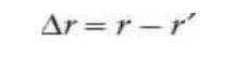
• Dlta r: the amount of lens distortion

• R: the radial distance from the principal point.

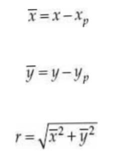
R is computed from the coordinates that are relative to the principal point. After converting an image point coordinate using the following equations:

• K1, k2, k3, k4: are coefficients of the polynomial. (Solved by the least squares).

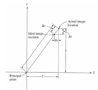
After the radial lens distortion value (delta r) is computed, its component for x , y (corrections) are calculated and subtracted from the coordinate:

subtracting the radial lens distortion can be done by using these equation:

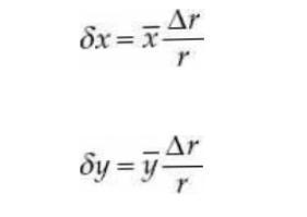
And corrected coordinates computed from:

5. Correction for Atmospheric Refraction:

Photogrammetric equations are based on an assumption that light rays travel in straight lines, and that is not correct because as it known that the density and refraction index decreases with increasing altitude, and according to Snell’s law, light rays bent through the atmosphere. So that a correction needed to eliminate the effect of refraction. If it ignored the light will appear to be coming from a false point as shown in the figure below:

The usual approach to correct the atmospheric refraction effect is based on an assumption that the refraction index of air is directly proportional to the height. Snell’s low can be solved along the path of the ray. The angular distortion is computed from the equation:

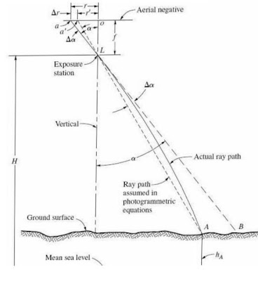
• Alpha: the angle between vertical and the ray of light.

• K: a valued depend on the flying height and elevation of object point. K’s unite is in degree. K in a standard atmosphere can be computed from:

• H: flying height of the camera above the mean sea level in kilometre.

• (h): elevation of object point above the mean sea level.

First we need to calculate the radial distance r in order to compute the corrected atmospheric effect point coordinate. R is computed from:

Also:

Then substitute the value of K and tan alpha in the angular distortion equation:

Then the radial distance from the principal point to the corrected image coordinate, and the change in the radial distance can be computed from:

Finally corrected coordinates from the atmospheric effect can be calculated from the same equations derived in the lens distortion correction: 

And the corrected coordinates:

6. Correction for Earth Curvature:

The points are referenced to approximately curved surface (mean sea level) while photogrammetric equations are based on an assumption that points are referenced to a plane surface, So that a correction for the earth curvature is applied.

Although, it has been recognized that earth curvature correction is theoretically wrong. However, it also has been accepted because it was proven practically that it is better to apply the correction and it leads to more accurate results rather than ignoring it.

The main problem with the earth curvature correction is it will degrade the accuracy of either the X or Y object space coordinate, because of the nature of the map projection.

When employing a three-dimensional orthogonal object space coordinate system, will avoid any need for earth curvature correction. So the earth curvature will be a normal characteristic od the terrain and will be solve as a topographic feature.

Measurement of Feature Positions and Edges:

Since the point must be visible in a photograph to be measure, the object must have a finite size. The cover of a manhole will appear as ideal point feature as long as scale of the image is not too large. Under magnification or image zoom in, the centre of the point will be clearly visible although the edge may not, in many cases it is necessary to practically measure the edges when mapping features. And some errors maybe expected.